
Introduction
The CU EMP lab is equipped with a JEOL 8230 Superprobe; this instrument was acquired and installed 2016 with the support of an NSF MRI grant and a cost matching contribution from CU Boulder. This state of the art instrument is equipped with five wavelength dispersive spectrometers. Four of these spectrometers are outfitted with JEOL large area (L-type) monochromator crystals which yield x-ray count rates that are a factor of 2-3 higher than standard J-type spectrometers. The L-type spectrometers provide enhanced instrument sensitivity which greatly improves the performance of the instrument in the analysis of trace elements (concentrations <500ppm). The instrument is also equipped with a Thermo UltraDry energy dispersive x-ray spectrometer (EDS) and a panchromatic cathodoluminescence detector. The JEOL 8230 vacuum system is completely dry-pumped, employing a combination of a scroll pump (roughing), turbo molecular pump (hi-vac), and sputter ion pump (electron gun assembly); this vacuum system eliminates hydrocarbon contamination on polished sample surfaces during long beam exposures. The lack of hydrocarbon contamination produces optimal conditions for the accurate analysis of light elements (Z<9) and trace elements.
Quantitative WDS Analysis: How It Works In a Nutshell
The primary function of the EMP is to provide in-situ quantitative chemical analyses via wavelength dispersive x-ray spectrometry (WDS). Samples bombarded by high energy electrons emit both characteristic x-rays and continuum or bremmstrahlung radiation. Characteristic x-rays are generated when high energy electrons (10-25 KeV) from the primary beam in-elastically collide with and eject electrons in core level orbitals; the “core holes” generated in this way are highly unstable and are rapidly filled with an electron from a higher energy orbital (e.g., a 2p electron replacing a vacancy in a core level 1s orbital). This energy level transition by the filling electron results in the emission of an x-ray with a wavelength that is inversely proportional to the energy difference between two orbitals involved in the transition. The wavelength of characteristic x-rays produced in manner scales with the Z number of the emitting element, such that elements higher Z elements have emit x-rays with shorter wavelengths and higher energy. In this way, the wavelength of characteristic x-rays generated from a particular (i.e., discrete) electron transition serve as a “fingerprint” that can be used to identify the presence of a given element. The effect of Z on the x-ray wavelength can be illustrated by considering the generated by the 1s-2p electron transition (i.e., Kα line) for Fe and Ni. The Kα emission wavelength for Fe (Z=26) is 1.935 angstroms, whereas the Kα emission wavelength for Ni (Z=28) is 1.657 angstroms.

The wavelength dispersive spectrometers allow us isolate, collect, and measure the intensity of photons with a specific wavelength (via Bragg diffraction -) with a high degree of energy resolution. Using this method, a spectrometer can be “tuned” to the wavelength of a characteristic x-ray emission from an element of interest. The tuning of the spectrometer effectively filters out a cacophony of x-ray photons of different wavelengths that are also simultaneously generated from the sample (i.e. characteristic x-rays from other elements present and background/bremmstrahlung radiation). Separated characteristic x-rays photons of interest collected and accurately counted using a gas proportional detector. The emission intensity (counts per unit time) for given characteristic x-ray line is proportional its concentration in the sample. Measured x-ray intensities are corrected for “matrix” effects and converted concentrations using a sophisticated, iterative correction algorithm ( dont worry, this is done by computer!). The accurate conversion of measured x-ray intensity into quantitative chemical information requires the consideration of what are known as “matrix” effects. The generation and emission of characteristic x-rays are not exclusively controlled by the concentration of the element of interest, but also influenced by the composition of the sample “matrix”. Factors and processes such as electron such as electron backscatter efficiency, attenuation/absorption of generated x-rays within the specimen itself, and secondary fluorescent X-ray emission, collectively affect the observed emission intensity for a given characteristic x-ray line. These matrix effects are described quantitatively by what are known as the ZAF coefficients.
A full description of data reduction, matrix corrections, and counting statistics is well beyond the scope of the description on this website, so of this cursory explanation doesn’t satisfy your curiosity, a excellent theoretical discussion of all of these topics can be found in “Electron Microprobe Analysis” by S.H.J. Reed – Cambridge Monographs on Physics (Cambridge Press).
Detection Limits and Analytical Sensitivity of Quantitative WDS Analysis
Minimum detection limits for quantitative EMP analyses obtained under “standard” EPMA analytical conditions (15 KeV and beam currents from 20nA-50nA) typically range from 150 ppm to 300 ppm at the 3σ level (or 99.7% confidence interval). For trace elements, the detection can be pushed down to values as low as 10-50 ppm by employing extended peak and background counting times and using an elevated beam current. Analytical conditions can be customized/optimized to achieve the detection limits required for your specific application, so please contact the lab manager to discuss what we can do for you and your project!
The analytical sensitivity for most major elements ranges from 1.00%-0.50% relative. To illustrate the significance these values, consider the EMP measured concentration of Mg in a crystal of San Carlos olivine (SCO is a well characterized EMP standard reference material that is derived from a suite of mantle spinel lherzolite xenoliths from San Carlos AZ). The measured elemental Mg concentration of the SCO crystal would reported as 29.75 wt % ± 0.145 wt%. In other word each point analysis can statistically distinguish differences in Mg concentration of ~ 1500ppm. In terms terms of a structural mineral formula, this translates to 1.853 ± 0.004 cations of Mg2+ per olivine formula unit – or a precision of better than 2 cations in a thousand (two per mil). As such, WDS spot analyses can be a powerful tool for quantifying subtle chemical zoning in inhomogeneous materials (single crystals or otherwise). Under some circumstances the analytical precision/sensitivity can be increased further by manipulating beam current and spectrometer counting times to increase the number of x-ray photons counted by the detectors.
Samples and Sample Preparation
High quality quantitative analysis requires flat, well polished specimens. High quality sample preparation is critical for obtaining high quality quantitative results. For most geological/mineralogical applications this typically consists of a petrographic thin section that has been specially polished to a 0.50 micron finish. The sample holder/stage can accommodate 25mm diameter round thin sections or standard 27mm by 46mm rectangular petrographic thin section. Up to four 27mm by 46mm sections and as many as nine 25mm round sections can be loaded into the instrument simultaneously

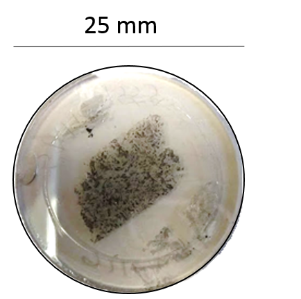
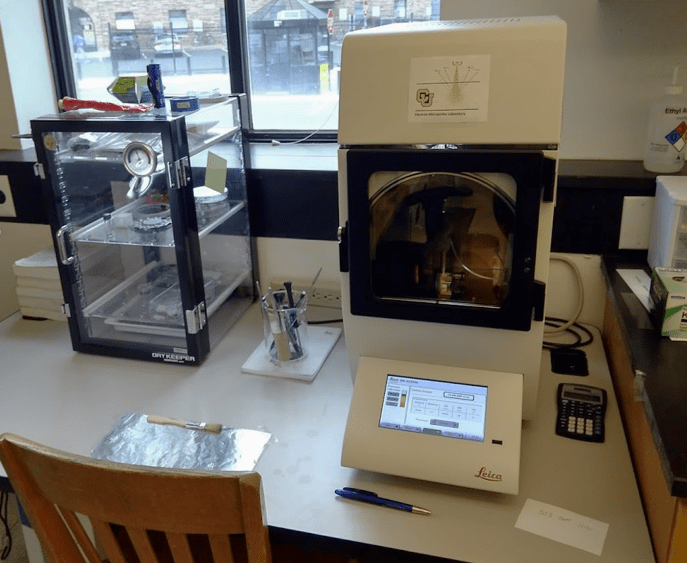
For non-geological samples, specimens can be mounted in 25mm or 30mm epoxy wafers and polished to the appropriate specification. Non electrically conductive samples (i.e., silicates) must be coated with thin film of conductive material. For quantitative analysis a carbon thin film of 15-20 nm (~100-150 carbon atoms thick!) thick is typically deposited thermal pulse evaporation. The EMP laboratory is equipped with at Leica ACE600 high vacuum carbon evaporator which is capable of depositing and measuring carbon thin films with an accuracy of +/- 1 nm.
Other Information Derived from WDS
For some elements, additional information about their valence and bonding/coordination environment can be obtained WDS spectra. A classic example of this effect can be illustrated centriod energy the sulfur Kα x-ray line. The energy of the S Kα x-ray depends on the formal valence of sulfur in the material being analyzed. When sulfur is present as the S2- anion, the centriod is shifted to lower energies than when it is present as the S6+ cation bonded in oxygen in a sulfate complex.
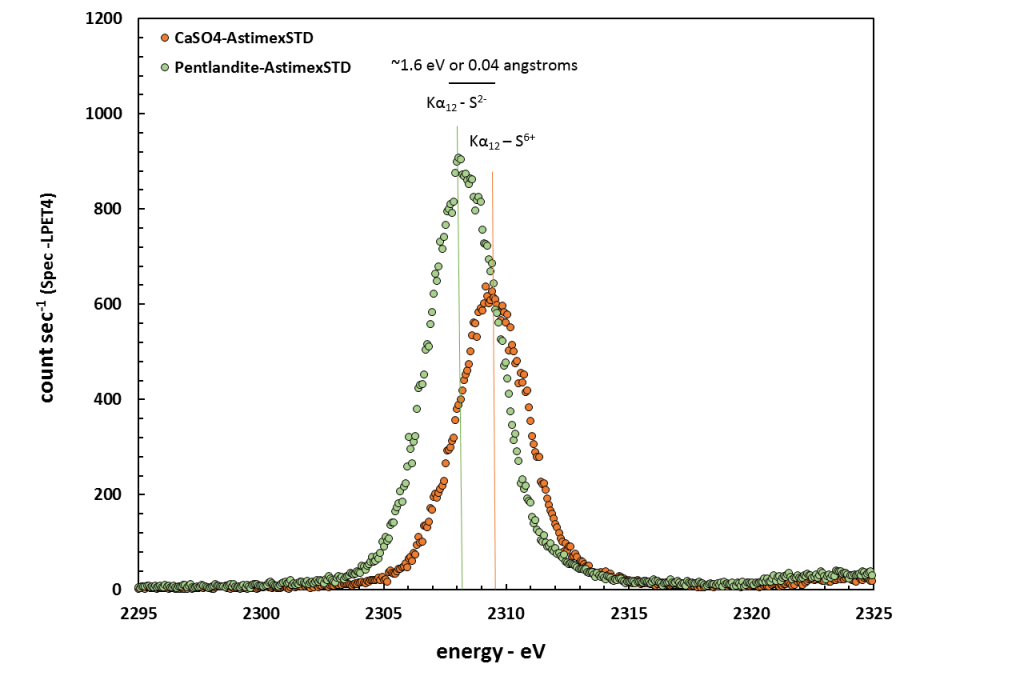
The plot of WDS spectra for pentlandite (NiS) and anhydrite (CaSO4) shown below illustrates this effect (shown in energy space rather than wavelength). Concerting eV to wavelength in angstroms, the S Kα centroid measured for NiS is 5.371 angstroms whereas the S Kα centroid measured for CaSO4 is 5.368 angstroms. This corresponds to an energy difference of about 1.6 eV and is a fantastic illustration of the superior ability of the WD spectrometers to resolve extremely small wavelength differences.
WDS Element Mapping
Maps of element distribution can also be produced using the WDS spectrometers. The image below is a false-colored and annotated Fe Kα x-ray map of the phase assemblage in the “basaltic” meteorite Sahara 99555 (SAH 99555 is classified as an angrite and is one of the oldest igneous rocks in the solar system at 4.55 Ga).
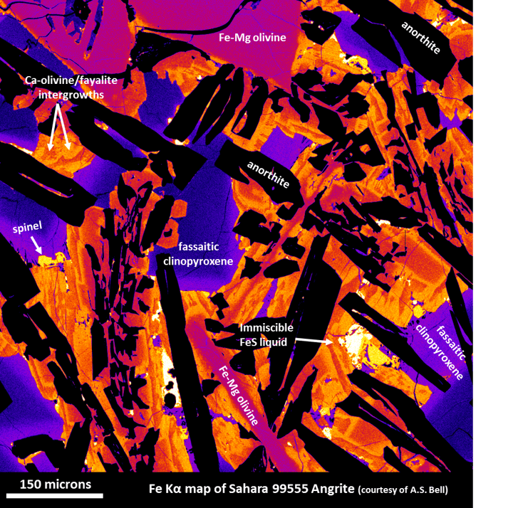
The warmer colors correspond to higher measured Fe Kα intensity (per pixel) and thus can be inferred as areas of higher Fe concentrations; conversely cool colors correspond to lower measured Fe Kα intensity thus lower Fe concentrations. Maps of similar dimensions and pixel (1 μm2 per pixel) resolution can be collected for up to five elements simultaneously in ~1-2hrs.
